Bayesian Meta-Analysis with R and Stan
Overview
Meta-analysis is frequently used to summarize results from multiple research studies. Since studies can be thought of as exchangeable, it is natural to analyze them using a hierarchical structure.
This page uses a Bayesian hierarchical model to conduct a meta-analysis of 9 randomized controlled trials (RCTs) of breast cancer screening. The analysis first replicates the frequentist results reported by Marmot et al. and then reexamines them in a Bayesian framework. The RCTs used in the meta-analysis are summarized in more detail by Gøtzsche et al..
R and Stan code for the analysis can be found here and here.
Previous RCTs and Relative Risks
We begin by placing data from previous trials into a data frame using the summaries provided by Gøtzsche et al.. The treatment (group 1) is screening with mammography and the control (group 0) is no screening. The outcome in the treatment and control groups for study \(j\), \(d_{1j}\) and \(d_{0j}\) respectively, is the number of breast cancer deaths during 13 years of follow up for women at least 50 years of age. There are \(n_{1j}\) and \(n_{0j}\) patients in the treatment and control groups respectively.
rct <- data.frame(study = c("New York", "Malamo I", "Kopparberg", "Ostergotland",
              "Canada I", "Canada II", "Stockholm", "Goteborg", "UK age trial"))
rct$year <- c(1963, 1976, 1977, 1978, 1980, 1980, 1981, 1982, 1991)
rct$d1 <- c(218, 87, 126, 135, 105, 107, 66, 88, 105)
rct$n1 <- c(31000, 20695, 38589, 38491, 25214, 19711, 40318, 21650, 53884)
rct$d0 <- c(262, 108, 104, 173, 108, 105, 45, 162, 251)
rct$n0 <- c(31000, 20783, 18582, 37403, 25216, 19694, 19943, 29961, 106956)
The relevant statistic for the meta-analysis is the relative risk ratio, or \(p_{1j}\)/\(p_{0j}\), where \(p_{1j} = d_{1j}/n_{1j}\) and \(p_{0j} = d_{0j}/n_{0j}\). We work with the log of the relative risk ratio, \(y_j = log(p_{1j}) - log(p_{0j})\), because it is approximately normally distributed even in relatively small samples. We can calculate the variance of each term of \(y_j\) by treating \(p_{1j}\) and \(p_{0j}\) as sample proportions and using the delta method, so that the variance of \(y_j\) is,
\[\begin{aligned} \sigma^2_j &\approx \frac{1 - p_{1j}}{n_{1j}p_{1j}} + \frac{1 - p_{0j}}{n_{0j}p_{0j}}. \\ \end{aligned}\]We can then calculate a point estimates for the relative risk in each study as well as a 95 percent confidence interval.
rct$p1 <- rct$d1/rct$n1
rct$p0 <- rct$d0/rct$n0
rct$rr <- rct$p1/rct$p0
rct$lrr <- log(rct$rr)
rct$lse <- sqrt((1 - rct$p1)/(rct$p1 * rct$n1) + (1 - rct$p0)/(rct$p0 * rct$n0))
rct$lower <- exp(rct$lrr - qnorm(.975) * rct$lse)
rct$upper <- exp(rct$lrr + qnorm(.975) * rct$lse)
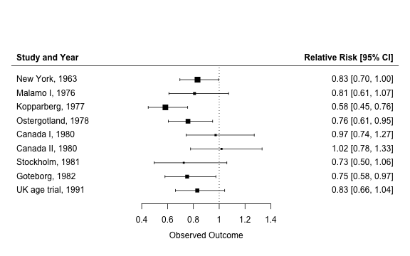
The results can be visualized nicely by creating a forest plot with the metafor package.
library("metafor")
p <- forest(x = rct$rr, ci.lb = rct$lower, ci.ub = rct$upper,
       slab = paste(rct$study, rct$year, sep = ", "), refline = 1)
text(min(p$xlim), .88 * max(p$ylim), "Study and Year", pos = 4, font = 2)
text(max(p$xlim), .88 * max(p$ylim), "Relative Risk [95% CI]", pos = 2, font = 2)

Hiearchical Model
The results from the separate RCTs can be modeled using a hierarchical model. We use the fact that the log of the relative risk is approximately normally distributed and assume that the random effects follow a normal distribution,
\[\begin{aligned} y_j &\sim N(\theta_j, \sigma^2_j) \\ \theta_j &\sim N(\mu, \tau), \end{aligned}\]where \(\sigma^2_j\) is assumed to be known with certainty (this assumption is not problematic because the binomial variances in each study are estimated precisely due to the large sample sizes). Meta-analyses are typically concerned with the overall mean, \(\mu\).
There are, in general, three ways to estimate the random effects, \(\theta_j\).
- No-pooling: there is a separate model for each study and \(\theta_j=y_j\). This is a special case of the hierarchical model in which \(\tau = \infty\).
- Complete-pooling: patients in each study are random samples from a common distribution so \(\theta_j = \mu\). This is a special case of the hierarchical model in with \(\tau = 0\).
- Partial-pooling: the hierarchical model is a compromise between the no-pooling and the complete-pooling estimates. In this case \(\tau\) is unknown and \(\theta_j\) is closer to \(\mu\) when \(\tau\) is small relative to \(\sigma^2_j\), and closer to \(y_j\) when the reverse is true.
Estimation
No-pooling Estimates
A fixed-effect meta-analysis model completely pools the relative risk estimates across studies. The overall mean is commonly estimated by taking an inverse-variance weighted average of studies. This can be done in using the rma function in the metafor package.
me.fe <- rma(rct$lrr, rct$lse^2, method = "FE")
c(exp(me.fe$b), exp(me.fe$ci.lb), exp(me.fe$ci.ub))
## [1] 0.8041868 0.7406291 0.8731987
The relative risk and 95 percent confidence intervals are identical to the fixed-effect meta-analysis results reported in Gøtzsche et al.. We can check to see that the point estimate is identical to taking a weighted average of the relative risks in the RCTs.
exp(weighted.mean(rct$lrr, 1/(rct$lse^2)))
## [1] 0.8041868
Maximum Likelihood Estimation
A hierarchical model applied to meta-analysis is typically referred to as a random-effect meta-analysis model in the medical literature. The parameters of the hierarchical model can be estimated in either a frequentist or a Bayesian framework. In a frequentist setup, point estimates (rather than probability distributions) for the parameters are estimated. This can be done in a number of ways, but here we will estimate the parameters with restricted maximum likelihood (REML) using the rma function.
me.re <- rma(rct$lrr, rct$lse^2)
c(exp(me.re$b), exp(me.re$ci.lb), exp(me.re$ci.ub))
## [1] 0.8029497 0.7259418 0.8881267
This analysis reproduces the results reported by Marmot et al..
Bayesian Estimation
One problem with the maximum likelihood approach is that it does not account for uncertainty in \(\tau\) and produces confidence intervals for \(\mu\) that are too narrow. A Bayesian model that produces complete probability distributions for each parameter can be estimated using the probabilistic programming language Stan. We begin by preparing the data.
library("rstan")
set.seed(101)
J <- nrow(rct)
stan.dat <- list(J = J, y = rct$lrr, sigma = rct$lse)
Next we specify the model. Note that we can rewrite the upper-level model as \(\theta_j = \mu + \tau \eta\) where \(\eta \sim N(0, 1)\), which speeds up the Stan code. Furthermore, \(\mu\) and \(\tau\) are given uniform priors.
data {
  int<lower=0> J; // number of trials
  real y[J]; // estimated log relative risk
  real<lower=0> sigma[J]; // se of log relative risk
}
parameters {
  real mu;
  real<lower=0> tau;
  real eta[J];
}
transformed parameters {
  real theta[J];
  for (j in 1:J)
    theta[j] = mu + tau * eta[j];
}
model {
  eta ~ normal(0, 1);
  y ~ normal(theta, sigma);
}
We fit the model and extract samples from the joint posterior distribution.
fit <- stan(file = "_rmd-posts/bayesian_meta_analysis.stan",
            data = stan.dat, iter = 2000, chains = 4)
post <- extract(fit, permuted = TRUE)
As expected, the 95 percent credible interval for the exponential of the overall mean is slightly wider that the 95 percent confidence interval produced using REML.
quantile(exp(post$mu), probs = c(.025, .5, .975))
##      2.5%       50%     97.5%
## 0.6889931 0.8011223 0.9110904
This addditional uncertainty comes from averaging over \(\tau\), which has a rather wide probability distribution.
quantile(post$tau, probs = c(.025, .5, .975))
##        2.5%         50%       97.5%
## 0.006847247 0.102239111 0.337733161
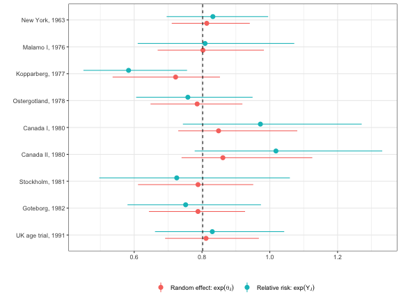
The effects, \(\theta_j\), are shrunk toward the overall mean, \(\mu\). The following plot examines the degree of shrinkage by comparing the effects from the Bayesian model to the relative risks when each study is analyzed separately.
library("ggplot2")
theme_set(theme_bw())
p.dat <- apply(exp(post$theta), 2, quantile, probs = c(.025, .5, .975))
p.dat <- data.frame(lower = p.dat[1, ], rr = p.dat[2, ], upper = p.dat[3, ])
p.dat <- rbind(p.dat, rct[, c("lower", "upper", "rr")])
p.dat$lab <- rep(c("Theta", "Y"), each = J)
p.dat$id <- rep(seq(9, 1), 2)
p.dat$idlab <- factor(p.dat$id, labels = rev(paste(rct$study, rct$year, sep = ", ")))
p.dat$yint <- mean(exp(post$mu))
ggplot(p.dat, aes(x = idlab, y = rr, ymin = lower, ymax = upper, col = lab)) +
  geom_pointrange(aes(col = lab), position = position_dodge(width = 0.50)) +
  coord_flip() + geom_hline(aes(yintercept = yint), lty = 2) +  xlab("") +
  ylab("")  + theme(legend.position="bottom") +
  scale_colour_discrete(name="",
                        labels = c("Theta" = bquote("Random effect:"~exp(theta[J])~" "),
                                    "Y"= bquote("Relative risk:"~exp(Y[J]))))

There is considerable shrinkage and the degree of shrinkage is larger for studies where the relative risks are estimated less precisely. The 95 percent credible intervals using the Bayesian approach are also narrower than the 95 percent confidence intervals from the individual studies because the hierarchical model pools information across RCTs
Although most meta-anlayes focus on the overall mean, there are other quantities of interest that may be more meaningful. For example, it might me more useful to predict the effect of mammography screening in a new population by making a prediction about a new study effect, say \(\tilde{\theta}_j\), rather than from \(\mu\). Predictions in a new population can be made very easily in a Bayesian framework because the study effects are assumed to be exchangable; that is, we can simulate the posterior distribution of \(\tilde{\theta_j}\) by drawing \(\tilde{\theta}_j \sim N(\mu, \tau)\) using the values of \(\mu\) and \(\tau\) drawn from the posterior simulation.
n.sims <- nrow(post$mu)
theta.new <- rep(NA, n.sims)
for (i in 1:n.sims){
  theta.new[i]  <- rnorm(1,  post$mu[i],  post$tau[i])
}
Although the posterior medians are similar, the 95 percent credible interval for \(exp(\tilde{\theta}_j)\) is much wider than for \(exp(\mu)\).
quantile(exp(theta.new), probs = c(.025, .5, .975))
##      2.5%       50%     97.5%
## 0.5711096 0.8017504 1.1106414