Probabilistic Sensitivity Analysis with R
- Overview
- Normal distribution
- Multivariate normal distribution
- Beta distribution
- Dirichlet distribution
- Gamma and lognormal distributions
- Uniform distribution
- Performing a PSA
Overview
Decisions to adopt or reimburse health technologies are often guided by cost-effectiveness analyses. The outcomes needed to conduct cost-effectiveness analyses are simulated using decision-analytic models, which combine information from multiple sources and extrapolate outcomes beyond the time horizons or settings from the available evidence. These models are subject to a number of sources of uncertainty, including parameter uncertainty.
The standard methodology for quantifying the impact of parameter uncertainty is probabilistic sensitivity analysis (PSA), which propagates uncertainty in the model input parameters throughout the model by randomly sampling the input parameters from suitable probability distributions. Probability distributions are determined according to the distributional properties of the statistical estimates, which, in turn, depend on the statistical techniques used and the distributions of the underlying data
R, which is designed specifically for statistical computing, may be the most natural programming language for performing PSA. Random samples can be drawn from almost any probability distribution using R. Below, we examine different probability distributions, and show how they can be used to sample parameter types that are commonly used in cost-effectiveness modeling.
Normal distribution
Cost-effectiveness analysis is typically concerned with mean outcomes in a given patient population. The normal distribution is therefore particularly attractive, because the central limit theorem establishes that in relative large samples, the sample mean is approximately normally distributed even if the underlying probability distribution is not.
set.seed(100)
norm.sample <- rnorm(n = 1000, mean = 10, sd = 2)
library("ggplot2")
theme_set(theme_bw())
ggplot2::ggplot(data.frame(x = norm.sample), aes_string("x")) +
  geom_histogram(color = "white", fill = "dodgerblue3", binwidth = .4)
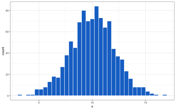
In health economics, normal distributions can be used to summarize the distribution of continuous outcomes, such as the parameter estimates of a simple linear regression. However, the normal distribution only applies to a single variable and in most real-world cases, it will be necessary to sample multiple correlated random variables.
Multivariate normal distribution
The multivariate normal distribution is a generalization of the univariate normal distribution. It is a particularly useful distribution in statistics because the multivariate normal distribution can be used to describe, at least approximately, parameters from regression models due to the multivariate central limit theorem.
Decision-analytic models rely heavily on estimates from regression models. For example, time to treatment discontinuation and patient survival are estimated using survival models, which can extrapolate outcomes beyond the available follow-up data. Below, we illustrate by estimating a Weibull model with the flexsurv package.
library("flexsurv")
surv.fit <- flexsurvreg(Surv(recyrs, censrec) ~ 1, data = flexsurv::bc, dist = "weibull")
The shape and scale parameters can be sampled with a multivariate normal distribution using the function mvrnorm from the package MASS.
library("MASS")
coef.sample <- MASS::mvrnorm(n = 1000, mu = surv.fit$res.t[, "est"], surv.fit$cov)
ggplot2::ggplot(data.frame(coef.sample), aes_string(x = "shape", y = "scale")) +
  geom_point()
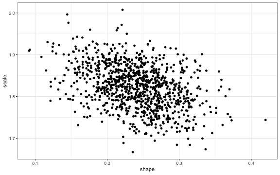
The points are downward sloping because the scale and shape parameter are negatively correlated.
Beta distribution
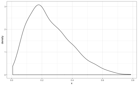
The beta distribution is appropriate for describing the distribution of a probability or proportion. For instance, the beta distribution could be used to model the uncertainty of probabilities in a decision tree.
In Bayesian statistics, the beta distribution is a conjugate prior for the binomial distribution. The binomial distribution is a discrete probability distribution for number of successes in $n$ trials where the probability of each outcome being a success is $\pi$, defined on [0,1]. The beta distribution is parameterized by two positive shape parameters, $\alpha$ and $\beta$. Letting $y$ denote the number of successes, we can define a model where the priors and likelihood are,
\[\begin{aligned} p(\pi |\alpha, \beta) = \text{Beta}(\alpha, \beta) \\ p(y | \pi) = \text{Bin}(n, \pi). \end{aligned}\]The posterior distribution for $\pi$ is given by
\[p(\pi|y, \alpha, \beta) = \text{Beta}(\alpha + y, \beta + n - y).\]It is therefore straightforward to characterize the posterior distribution of $\pi$ when counts of successes and failures are available. But in many applications—such as meta-analysis or use of secondary data sources—this will not be the case. Still, in these cases, the posterior distribution of $\pi$ can be estimated using the method of moments as long as sample means/proportions and standard errors are reported. The mean of the beta distribution is $\alpha/(\alpha + \beta)$ and the variance is $\alpha \beta/(\alpha + \beta)^2(\alpha + \beta + 1)$. Thus, if $\overline{x}$ is the sample mean and $s^2$ is the sample variance, we can solve for $\alpha$ and $\beta$ as,
\[\begin{aligned} \alpha = \overline{x}\left(\frac{\overline{x}(1-\overline{x})}{s^2} - 1 \right) \\ \beta = \left(1 - \overline{x}\right)\left(\frac{\overline{x}(1-\overline{x})}{s^2} - 1 \right), \end{aligned}\]with $s^2 < \overline{x}(1-\overline{x})$. We can write a short function, beta_mom, to calculate $\alpha$ and $\beta$ using the method of moments.
beta_mom <- function(mean, var){
  term <- mean * (1 - mean)/var - 1
  alpha <- mean * term
  beta <- (1 - mean) * term
  if (var >= mean * (1 - mean)) stop("var must be less than mean * (1 - mean)")
  return(list(alpha = alpha, beta = beta))
}
beta.pars <- beta_mom(mean = .25, var = .02)
The sample proportion, $\pi$, can then be sampled using the functionrbeta.
pi.sample <- rbeta(n = 1000, shape1 = beta.pars$alpha, shape2 = beta.pars$beta)
mean(pi.sample)
## [1] 0.2525319
var(pi.sample)
## [1] 0.01983982
ggplot2::ggplot(data.frame(x = pi.sample), aes_string("x")) +
  geom_density()
Dirichlet distribution
The Dirichlet distribution is a multivariate generalization of the beta distribution. In Bayesian statistics, the Dirichlet distribution is used as a conjugate prior to the multinomial distribution. It is particularly useful in decision-analytic modeling because it can be used to characterize the distribution of transition probabilities.
The multinomial distribution is a discrete probability distribution for the number of successes for each of $k$ mutually exclusive categories in $n$ trials. The probabilities of the categories are given by $\pi_1,\ldots, \pi_k$, with $\sum_{j=1}^k \pi_j$ = 1 and each $\pi_j$ defined on [0,1]. The Dirichlet distribution is parameterized by the concentration parameters $\alpha_1,\ldots, \alpha_k$ with $\alpha_j > 0$. Letting $x_1,\ldots, x_k$ denote the number of successes in each category, the prior distribution and likelihood are,
\[\begin{aligned} p(\pi_1,\ldots,\pi_k |\alpha_1,\ldots, \alpha_k) = \text{Dirichlet}(\alpha_1,\ldots,\alpha_k) \\ p(x_1,\ldots,x_k | \pi_1,\ldots,\pi_k) = \text{Multin}(n, \pi_1,\ldots,\pi_k). \end{aligned}\]The posterior distribution for $\pi_1,\ldots,\pi_k$ is given by,
\[p\left(\pi_1,\ldots,\pi_k| x_1,\ldots,x_k, \alpha_1,\ldots,\alpha_k \right) = \text{Dirichlet}\left(\alpha_1 + x_1, \ldots, \alpha_k + x_k\right).\]The sum of parameters of the prior distribution, $\alpha_1,\ldots, \alpha_k$, is a measure of the strength of the prior distribution and can be thought of as a “prior sample size”.
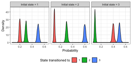
To illustrate use of the Dirichlet distribution for PSA, consider an example in which there are 3 states and individuals can transition between each of the states. Suppose that we observe the following number of transitions between the states: from state 1, the number of observed transitions to states 1, 2, and 3 are 200, 300, and 500, respectively; from state 2, the number of observed transitions to states 1, 2, and 3 are 100, 300, and 600, respectively; and from state 3, the number of observed transitions to states 1, 2, and 3 are 400, 100, and 500, respectively.
trans1 <- c(200, 300, 500)
trans2 <- c(100, 300, 600)
trans3 <- c(400, 100, 500)
trans <- matrix(c(trans1, trans2, trans3), ncol = length(trans1), byrow = TRUE)
head(trans)
##      [,1] [,2] [,3]
## [1,]  200  300  500
## [2,]  100  300  600
## [3,]  400  100  500
There are nine probabilities in the transition matrix,
\[\begin{pmatrix} \pi_{11} & \pi_{12} & \pi_{13} \\ \pi_{21} & \pi_{22} & \pi_{23} \\ \pi_{31} & \pi_{32} & \pi_{33} \end{pmatrix}.\]For each of the nine probabilities we set the prior, $\alpha_{11},\ldots,\alpha_{33}$ equal to 1, which is equivalent to a prior in which each transition is equally likely. We use the value 1 so that the prior has almost no influence on the posterior estimates for the transition matrix.
We can randomly sample transition probabilities using Dirichlet distributions with the function rdirichlet_mat from the hesim package (a package currently in active development by me). The function draws probabilities in each row in the transition matrix (i.e., transition probabilities from each state) from a separate Dirichlet distribution.
library("hesim")
alpha <- 1
tp.sample <- hesim::rdirichlet_mat(n = 1000, alpha + trans)
The distribution of transition probabilities for each of the 3 transitions in each of the 3 states are shown below.
tp.df <- data.frame(p = c(tp.sample),
                    cat = rep(c(rep("1", 3), rep("2", 3), rep("3", 3)),
                              dim(tp.sample)[3]),
                    state = rep(rep(paste0("Initial state = ", seq(1, 3)), 3),
                                dim(tp.sample)[3])
)
ggplot2::ggplot(tp.df, aes_string(x = "p", fill = "cat")) + geom_density() +
  facet_wrap(c("state"), nrow = 1) + theme(legend.position = "bottom") +
  scale_fill_discrete("State transitioned to") + xlab("Probability") + ylab("Density")
Gamma and lognormal distributions
The gamma and lognormal distributions are commonly used to model right skewed data. For example, both distributions are frequently used to model health care costs.
The gamma distribution can be parameterized using a shape parameter, $\kappa >0$, and a scale parameter, $\theta >0$. The mean and variance of the gamma distribution are $\kappa\theta$ and $\kappa \theta^2$, respectively. In applications where only secondary data is available, the gamma distribution can be parameterized using the method of moments given the sample mean, $\overline{x}$, and the sample variance, $s^2$,
\[\begin{aligned} \theta = \frac{s^2}{\overline{x}} \\ \kappa = \frac{\overline{x}}{\theta}. \end{aligned}\]We can write a function, gamma_mom, to estimate the shape and scale parameters using the method of moments,
gamma_mom <- function(mean, sd){
  if (mean > 0){
      theta <- sd^2/mean
      kappa <- mean/theta
  } else{
      stop("Mean must be positive")
  }
  return(list(kappa = kappa, theta = theta))
}
The lognormal distribution is parameterized by the mean, $\mu$, and the variance, $\sigma^2$, on the log scale. A random variable that is lognormally distributed is normally distributed on the log scale. The mean and variance of the distribution are given by $\exp(\mu + \sigma^2/2)$ and $[\exp(\sigma ^{2})-1]\exp(2\mu +\sigma ^{2})$, respectively. Like the gamma distribution, the parameters of the lognormal distribution can be parameterized using the method of moments if only summary level data is available,
\[\begin{aligned} \sigma^2 = \log\left[\frac{s^2 + \overline{x}^2}{\overline{x}^2}\right] \\ \mu = \log(\overline{x}) - \frac{1}{2}\sigma^2. \end{aligned}\]We write a function, lnorm_mom, to estimate the shape and scale parameters using the method of moments,
lnorm_mom <- function(mean, sd){
  if (mean > 0){
      sigma2 <- log((sd^2 + mean^2)/mean^2)
      mu <- log(mean) - 1/2 * sigma2
  } else{
      stop("Mean must be positive")
  }
  return(list(mu = mu, sigma2 = sigma2))
}
To illustrate the use of the gamma and lognormal distributions consider summary data with mean equal to $1,050$ and standard deviation equal to $500$, which are indicative of a right skewed distribution. We can estimate the parameters of the distributions using the method of moments.
mean <- 1050
sd <- 500
gamma.pars <- gamma_mom(mean, sd)
lnorm.pars <- lnorm_mom(mean, sd)
Lets check the mean and standard deviation of the distributions,
# mean
print(paste0("Mean of the gamma distribution: ",
             with(gamma.pars, kappa * theta)))
## [1] "Mean of the gamma distribution: 1050"
print(paste0("Mean of the lognormal distribution: ",
             with(lnorm.pars, exp(mu + sigma2/2))))
## [1] "Mean of the lognormal distribution: 1050"
# standard deviation
print(paste0("SD of the gamma distribution: ",
             with(gamma.pars, sqrt(kappa * theta^2))))
## [1] "SD of the gamma distribution: 500"
lnorm_sd <- function(mu, sigma2){
  sqrt((exp(sigma2) - 1) * exp(2 * mu + sigma2))
}
print(paste0("SD of the lognormal distribution: ",
             with(lnorm.pars, lnorm_sd(mu, sigma2))))
## [1] "SD of the lognormal distribution: 500"
To sample from the gamma and lognormal distributions, we can use the functions rgamma and rlnorm,
n <- 1000
gamma.sample <- rgamma(n, shape = gamma.pars$kappa, scale = gamma.pars$theta)
lnorm.sample <- rlnorm(n, meanlog = lnorm.pars$mu, sdlog = sqrt(lnorm.pars$sigma2))
sample.df <- data.frame(sim = c(gamma.sample, lnorm.sample),
                        dist = rep(c("Gamma", "Lognormal"), each = n))
ggplot2::ggplot(sample.df, aes_string(x = "sim", fill = "dist")) +
  geom_density(alpha = .4) + scale_fill_discrete("Distribution") +
  xlab("Simulated values") + ylab("Density")
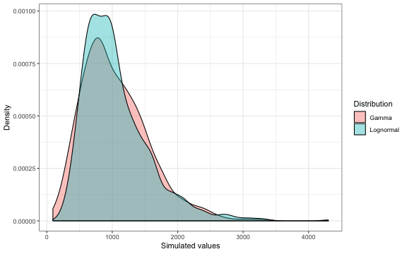
The distributions are similar, each being skewed with a long right tail, although the lognormal distribution has a higher peak.
Uniform distribution
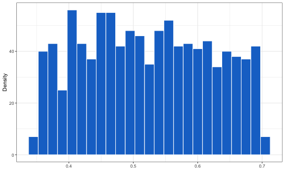
The uniform distribution is useful when there is little data available to estimate a parameter and determine its distribution. It is always preferable to place uncertainty on a parameter even when there is little evidence for it than to assume a fixed value (which gives a false sense of precision). Sampling from the uniform distribution is straightforward.
unif.sample <- runif(1000, .35, .7)
ggplot2::ggplot(data.frame(x = unif.sample), aes_string("x")) +
  geom_histogram(color = "white", fill = "dodgerblue3", binwidth = .015) +
  xlab("") + ylab("Density")
Performing a PSA
Although in theory, all the parameters in a decision-analytic model might be correlated, there is usually insufficient data to estimate these correlations. In practice, groups of parameters are sampled separately. For example, separate statistical models might be used to parameterize the distributions of the transition probabilities and the cost parameters. This is especially true in complicated simulation models with hundreds or thousands of parameters.
A rheumatoid arthritis individual patient simulation I developed provides an example of how parameters can be sampled in a complex model with R. In addition, my hesim package has a number of functions for summarizing a PSA as do the BCEA and the heemod packages.