Cost-effectiveness analysis with multi-state and partitioned survival models: hesim 0.2.0
Overview
hesim is an R package for health-economic simulation modeling and decision analysis. The most recent release, v0.2.0, is now on CRAN with new support for simulating partitioned survival models (PSMs) and continuous-time state transition models (CTSTMs). Documentation is provided on the package website.
Analyses are performed by constructing economic models that consist of (1) a disease model, (2) a utility model, and (3) cost models. A disease model simulates the progression of disease over time. In CTSTMs and PSMs this entails simulating the probability that patients are in mutually exclusive health states as a function of time. The utility model attaches utility values to the different health states and is used to compute quality-adjusted life-years (QALYs). Similarly, the cost models attach cost values to the health states for different categories of costs (e.g., drug costs, inpatient costs, outpatient costs, etc.).
Analyses follow a 3-step process consisting of (1) parameterization, (2) simulation, and (3) decision analysis. In the first step, statistical models are used to estimate the parameters of the economic model. In the second step, the parameterized economic model is simulated to compute quantities of interest—such as disease progression, QALYs, and costs—extrapolated over the desired time horizon (e.g., over a lifetime). Finally, in the third step, the simulated outcomes from step 2 are used to perform cost-effectiveness analyses (CEAs) and represent decision uncertainty.
The entire analysis is inherently Bayesian, as uncertainty in the parameters from the statistical models is propagated throughout the economic model and decision analysis with probabilistic sensitivity analysis (PSA). Since the simulations can be computationally intensive, the simulation code is written in C++ by leveraging Rcpp.
An example CTSTM
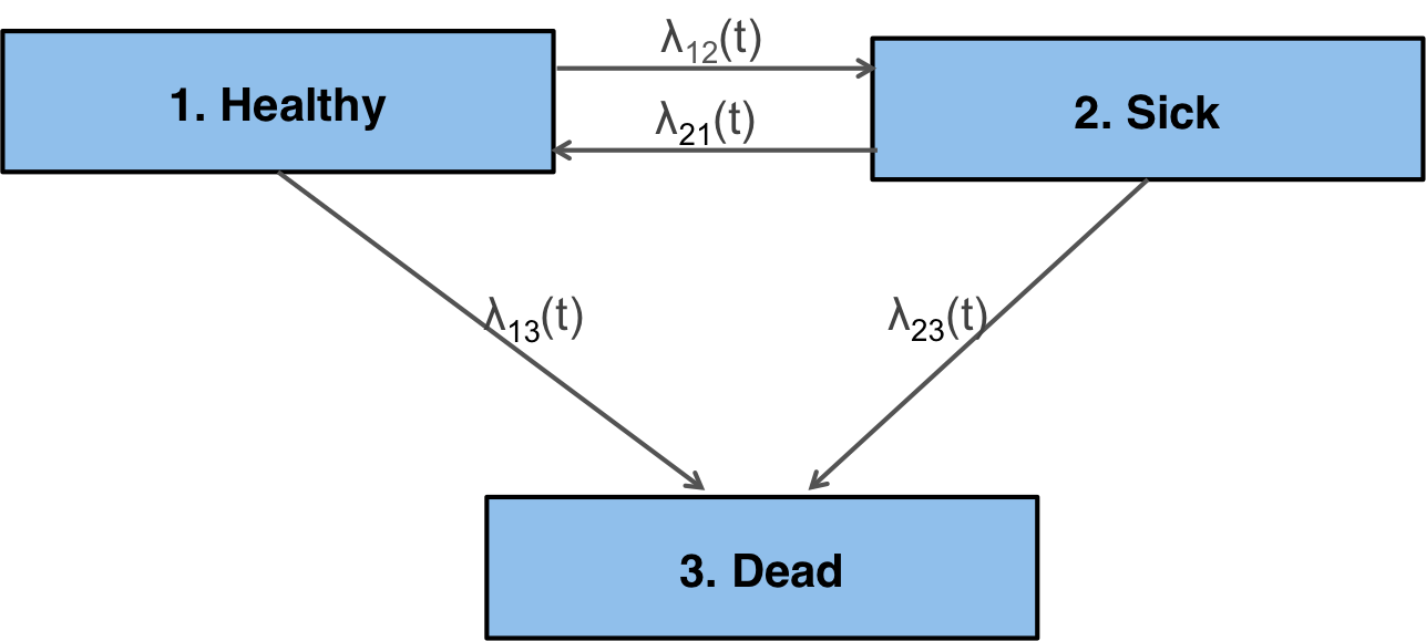
To illustrate, consider a reversible illness death model with 3 health states: (1) Healthy, (2) Sick, and (3) Dead.

There are 4 possible transitions—(1) Healthy to Sick, (2) Sick to Healthy, (3) Healthy to Dead, and (4) Sick to Dead—that are characterized by specifying a transition matrix. The transition from a state $r$ to a state $s$ is governed by a hazard function, $\lambda_{rs}(t)$, where $t$ is time.
tmat <- rbind(c(NA, 1, 2),
              c(3, NA, 4),
              c(NA, NA, NA))
colnames(tmat) <- rownames(tmat) <- c("Healthy", "Sick", "Dead")
print(tmat)
##         Healthy Sick Dead
## Healthy      NA    1    2
## Sick          3   NA    4
## Dead         NA   NA   NA
There are, in general, two possible timescales for the hazards. In a “clock forward” (i.e., Markov) model, time refers to time since entering the initial health state; conversely, in a “clock reset” (i.e., semi-Markov) model, time refers to time since entering the current state, meaning that time resets to 0 each time a patient enters a new state.
Decision problem and model setup
To setup an analysis in hesim, the competing treatment strategies, target population, and model structure must be specified. The specification of the target population will often depend on the model structure. For example, in a “clock reset” model, state occupancy probabilities can only be computed in a general fashion via individual-level simulation. This means that the simulated patient population must be large enough so that the results are not driven by random variation.
In this example, we will use a “clock reset” model to compare two treatment strategies in a population of size 1,000 that is 51 percent female with mean age of 45. The “data” is stored in an object of class hesim_data.
library("hesim")
library("data.table")
strategies <- data.table(strategy_id = c(1, 2))
n_patients <- 1000
patients <- data.table(patient_id = 1:n_patients,
                       age = rnorm(n_patients, mean = 45, sd = 7),
                       female = rbinom(n_patients, size = 1, prob = .51))
states <- data.table(state_id = c(1, 2),
                     state_name = c("Healthy", "Sick")) # Non-death health states
hesim_dat <- hesim_data(strategies = strategies,
                        patients = patients,
                        states = states)
Parameterization
The disease model is parameterized using a multi-state statistical model, which can be fit using the flexsurv package. We will fit a separate generalized gamma “clock reset” model for each transition with covariates for the treatment strategy and each patient’s age and gender.
library("flexsurv")
n_trans <- max(tmat, na.rm = TRUE) # Number of transitions
gg_fits <- vector(length = n_trans, mode = "list")
for (i in 1:length(gg_fits)){
  gg_fits[[i]] <- flexsurv::flexsurvreg(Surv(years, status) ~ factor(strategy_id) +
                                              age + female,
                                            data = ctstm3_exdata$transitions,
                                            subset = (trans == i) ,
                                            dist = "gengamma")
}
gg_fits <- flexsurvreg_list(gg_fits)
Mean utility and cost values can be attached to the health states using a stateval_tbl. In our PSA, we will assume that utility in each health state follows a beta distribution, which are parameterized using methods of moments after specifying the mean and standard errors.
utility_tbl <- stateval_tbl(data.table(state_id = states$state_id,
                                       mean = ctstm3_exdata$utility$mean,
                                       se = ctstm3_exdata$utility$se),
                            dist = "beta",
                            hesim_data = hesim_dat)
print(utility_tbl)
##    state_id mean        se
## 1:        1 0.65 0.1732051
## 2:        2 0.85 0.2000000
Drug costs are assumed to be known with certainty and vary by treatment strategy whereas medical costs vary by health state and are assumed to follow a gamma distribution.
drugcost_tbl <- stateval_tbl(data.table(strategy_id = strategies$strategy_id,
                                       est = ctstm3_exdata$costs$drugs$costs),
                            dist = "fixed",
                            hesim_data = hesim_dat)
medcost_tbl <- stateval_tbl(data.table(state_id = states$state_id,
                                       mean = ctstm3_exdata$costs$medical$mean,
                                       se = ctstm3_exdata$costs$medical$se),
                            dist = "gamma",
                            hesim_data = hesim_dat)
print(drugcost_tbl)
##    strategy_id   est
## 1:           1  5000
## 2:           2 10000
print(medcost_tbl)
##    state_id mean       se
## 1:        1 1000 10.95445
## 2:        2 1600 14.14214
Simulation
Constructing the economic model
To simulate quantities of interest, we must first construct the economic model by combining the disease, utility, and cost models (which are implemented as R6 classes). Since we are performing a PSA, we specify the number of desired PSA samples.
n_samples <- 1000
The disease (i.e., health state transition) model is a function of the parameters stored in gg_fits and input data. The input data for the transition model has one row for each treatment strategy and patient and includes the covariates used for prediction.
transmod_data <- expand(hesim_dat,
                        by = c("strategies", "patients"))
head(transmod_data)
##    strategy_id patient_id      age female
## 1:           1          1 51.53329      1
## 2:           1          2 41.32478      0
## 3:           1          3 57.70108      1
## 4:           1          4 45.58132      1
## 5:           1          5 47.77003      0
## 6:           1          6 29.64431      0
The transition model is fully specified by combining the fitted models and input data with the transition matrix, number of PSA samples, timescale, and starting age of each patient in the simulation (by default, patients are assumed to live no longer than age 100 in the individual-level simulation).
transmod <- create_IndivCtstmTrans(gg_fits, transmod_data,
                                      trans_mat = tmat, n = n_samples,
                                      clock = "reset",
                                      start_age = patients$age)
Since we are using mean models for utility and costs, they do not depend on covariates and therefore do not require input data.
# Utility
utilitymod <- create_StateVals(utility_tbl, n = n_samples)

# Costs
drugcostmod <- create_StateVals(drugcost_tbl, n = n_samples)
medcostmod <- create_StateVals(medcost_tbl, n = n_samples)
costmods <- list(Drug = drugcostmod,
                 Medical = medcostmod)
The economic model is constructed by combining the transition, utility, and cost models.
econmod <- IndivCtstm$new(trans_model = transmod,
                          utility_model = utilitymod,
                          cost_models = costmods)
Simulating outcomes
Disease progression (i.e, unique trajectories through the multi-state model) are simulated using the $sim_disease() method.
econmod$sim_disease()
head(econmod$disprog_)
##    sample strategy_id patient_id from to final time_start time_stop
## 1:      1           1          1    1  3     1   0.000000 10.495873
## 2:      1           1          2    1  2     0   0.000000  4.819635
## 3:      1           1          2    2  1     0   4.819635  5.320600
## 4:      1           1          2    1  2     0   5.320600  8.107048
## 5:      1           1          2    2  1     0   8.107048 10.775288
## 6:      1           1          2    1  2     0  10.775288 16.084566
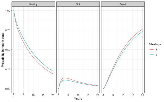
State occupancy probabilities at different time points are computed using $sim_stateprobs().
econmod$sim_stateprobs(t = seq(0, 20 , 1/12))

# Plot of state probabilities
library("ggplot2")
stprobs_mean <- econmod$stateprobs_[, .(prob_mean = mean(prob)),
                                     by = c("strategy_id", "state_id", "t")]
stprobs_mean[, state_name := factor(state_id,
                                    levels = 1:nrow(tmat),
                                    labels = rownames(tmat))]
ggplot(stprobs_mean, aes(x = t, y = prob_mean, col = factor(strategy_id))) +
  geom_line() + facet_wrap(~state_name) +
  xlab("Years") + ylab("Probability in health state") +
  scale_color_discrete(name = "Strategy") +
  theme(legend.position = "bottom") +
  theme_bw()

QALYs (and life-years) and costs are simulated using $sim_qalys() and $sim_costs(), respectively.
# QALYs (No discount rate and 3% discount rate)
econmod$sim_qalys(dr = c(0,.03))
head(econmod$qalys_)
##    sample strategy_id state_id dr    qalys       lys
## 1:      1           1        1  0 4.805071 12.311126
## 2:      1           1        2  0 2.502221  2.533594
## 3:      1           2        1  0 5.736869 14.698496
## 4:      1           2        2  0 2.037078  2.062618
## 5:      2           1        1  0 6.955268 12.724444
## 6:      2           1        2  0 1.895402  1.895427
# Costs (3% discount rate)
econmod$sim_costs(dr = 0.03)
head(econmod$costs_)
##    sample strategy_id state_id   dr category     costs
## 1:      1           1        1 0.03     Drug 42799.237
## 2:      1           1        2 0.03     Drug  8597.287
## 3:      1           2        1 0.03     Drug 99215.804
## 4:      1           2        2 0.03     Drug 13709.506
## 5:      2           1        1 0.03     Drug 44539.069
## 6:      2           1        2 0.03     Drug  6341.184
Cost-effectiveness analysis
The simulation output required for a CEA can be computed from an economic model by using the$summarize() method to compute mean costs and QALYs for each PSA sample.
ce_sim <- econmod$summarize()
The CEA is then performed using the icea() and icea_pw() functions, designed for individualized CEA (i.e., CEA by subgroup). The icea_pw() function performs pairwise CEA where all the interventions are compared to a comparator.
wtp <- seq(0, 300000, 500)
icea_out <- icea(ce_sim, k = wtp, dr_qalys = .03, dr_costs = .03)
icea_pw_out <- icea_pw(ce_sim, k = wtp, comparator = 1,
                       dr_qalys = .03, dr_costs = .03)
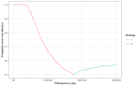
The output of these functions can be used to represent decision uncertainty using cost-effectiveness planes, cost-effectiveness acceptability curves (CEACs), cost-effectiveness acceptability frontiers (CEAFs), and the expected value of perfect information (EVPI). To illustrate, we will plot the CEAF, which shows the probability that the optimal treatment strategy (i.e., the strategy with the highest expected net monetary benefit) for a given willingness to pay for a QALY is cost-effective.
library("scales")
ggplot(icea_out$mce[best == 1], aes(x = k, y = prob, col = factor(strategy_id))) +
  geom_line() +
  xlab("Willingness to pay") +
  ylab("Probability most cost-effective") +
  scale_x_continuous(breaks = seq(0, max(wtp), 100000), label = scales::dollar) +
  theme(legend.position = "bottom") + scale_colour_discrete(name = "Strategy") +
  theme_bw()
