Two-part Models
- Overview
- Health Expenditure Data from the MEPS
- Model Choice
- Predicting Mean Expenditures
- Predictive Simulation
- Summary
Overview
Two-part models are often used to model strictly positive variables with a large number of zero values. They are consequently formulated as a mixture of a binomial distribution and a strictly positive distribution. I focus on continuous distributions for the positive values but two-part models—typically referred to as hurdle models—are used for count data as well. R code for the analysis can be found here.
Health Expenditure Data from the MEPS
Two-part models are commonly used to model healthcare expenditure data because a large fraction of patients don’t spend anything on medical care in a given time period. To see this, lets look at some real expenditure data from the Medical Expenditure Panel Survey (MEPS) 2012 Full Year Consolidated Data Files. The dataset can be found here. To speed up data manipulations, I recommend using the data.table package.
meps <- readRDS("data/meps-fyc-2012.rds")
Now lets plot the distribution of expenditures.
library(ggplot2)
theme_set(theme_bw())
qplot(totexp12, data = meps[totexp12 < quantile(meps$totexp12, probs = .95)])
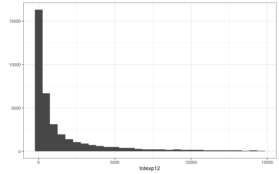
 The distribution of expenditures is heavily right skewed: there are many small values (the fraction of nonspenders is 0.24) and a few very large ones. This suggests 1) that a two-part model might be appropriate for this data and 2) that positive expenditures are not normally distributed. Common right skewed distributions that could be used to model positive expenditures include the lognormal distribution and the gamma distribution.
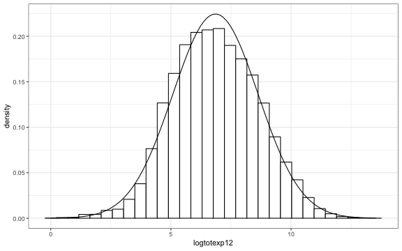
If the data is lognormally distributed, then the log of expenditures follows a normal distribution. We can investigate whether this is the case with the following plot. (Note that the syntax DT <- DT[...] is redundant but R Markdown prints the the output otherwise.)
library(MASS)
meps <- meps[, logtotexp12 := ifelse(totexp12 > 0, log(totexp12), NA)]
ggplot(meps, aes(x = logtotexp12)) +
  geom_histogram(aes(y = ..density..), colour = "black", fill = "White") +
  stat_function(fun = dnorm, args = fitdistr(meps[totexp12 > 0 , logtotexp12],
                                             "normal")$estimate)
 The data is approximately normally distributed, albeit skewed slightly to the left. Since the response variable is essentially normal, the error term in a linear regression model—or equivalently the response variable conditional on covariates—is likely approximately normal as well.
Model Choice
Two-part models can be easily estimated using separate regression models for the binomial distribution and the continuous distribution. The binomial component is typically modeled using either a logistic regression or a probit model. The continuous component can be modeled using standard ordinary least squares (OLS) or with generalized linear models (GLMs).
Different models for the continuous component can dramatically alter the results so model selection is important. This choice will depend on the goals of the analysis.
We saw that positive expenditures are very right skewed. If the data analyst is only concerned with modeling mean expenditures, then standard OLS on nontransformed expenditures might work fine regardless (as long as the OLS linearity assumption is satisfied). However, if the analyst needs to model the entire distribution of expenditures, then using a distribution that is appropriate for the data at hand is paramount.
Predicting Mean Expenditures
Before we begin we have to edit the variables in the MEPS to make them suitable for modeling. We model expenditures as a function of age, self-reported health status, race and ethnicity, and insurance status. A more accurate prediction model would also include variables containing detailed clinical information, but we will not consider clinical data here.
meps[, age := ifelse(age12x < 0, NA, age12x)]
meps[, age2 := age^2]
meps[, srh := as.factor(ifelse(rthlth53 < 0, NA, rthlth53))] # health status
meps[, hisp := ifelse(racethx == 1, 1, 0)] # hispanic race
meps[, black := ifelse(racebx == 1 | racebx == 2, 1, 0)]
meps[, prvins := ifelse(inscov12 == 1, 1, 0)] # private insurance
meps[, pubins := ifelse(inscov12 == 2, 1, 0)] # public insurance
meps[, d_totexp12 := ifelse(totexp12 == 0, 0, 1)] # indicator for positive spending
Lets subset our data set to exclude unnecessary variables and limit ourselves to non-missing observations.
meps[, id := seq(1, nrow(meps))]
xvars <- c("age", "age2", "srh", "hisp", "black", "prvins", "pubins")
meps <- meps[, c("id", "totexp12", "d_totexp12", "logtotexp12", xvars), with = FALSE]
meps <- meps[complete.cases(meps[, xvars, with = FALSE])]
To test our model we will estimate it on half of the data and then use the parameters to predict expenditures for the other half. To do so, we’ll create a randomly chosen variable indicating whether the respondent is in the training set or the test set.
set.seed(100)
meps[, sample := sample(c("train", "test"), nrow(meps), replace = TRUE)]
We fit the binary portion of the model using logistic regression. The continuous component is modeled in three different ways: with a simple OLS regression on spending in levels, with OLS on the log of spending, and with a gamma GLM. The gamma model is estimated with a log link function, which constrains the predicted means to be positive and ensures that mean expenditures are a linear function of the coefficients on the log scale.
Fm <- function(y, xvars){
  return(as.formula(paste(y, "~", paste(xvars, collapse = "+"))))
}
# part 1
logistic.fit <- glm(Fm("d_totexp12", xvars), meps[sample == "train"], family = binomial)

# part 2
ols.fit <- lm(Fm("totexp12", xvars), meps[totexp12 > 0 & sample == "train"])
logols.fit <- lm(Fm("logtotexp12", xvars), meps[totexp12 > 0 & sample == "train"])
gamma.fit <- glm(Fm("totexp12", xvars), meps[totexp12 > 0 & sample == "train"],
                 family = Gamma(link = log))
Using these models we can predict mean expenditures, $Y$, given a matrix of covariates, $X$, as follows,
\[\begin{aligned} E[Y|X] &= \Pr(Y >0|X)\times E(Y|Y>0, X). \end{aligned}\]The first term can be easily estimated using a logistic regression. The second term is easy to estimate if the expected value of $Y$ is being modeled directly. For instance, in a gamma GLM with a log link, we model the log of mean expenditures,
\[\begin{aligned} \log(E[Y])=X\beta, \end{aligned}\]where $\beta$ is the coefficient vector and we have suppressed the dependence of $E[Y]$ on $X$. We can therefore obtain the mean of expenditures by simply exponentiating $\log(E[Y])$. Things are less straightforward in the logtransformed OLS regression since we are modeling the mean of log expenditures,
\[\begin{aligned} E[\log(Y)]=X\beta, \end{aligned}\]and $E[\exp(\log(Y))] \neq \exp(E[\log(Y)])$. We can however estimate mean expenditures if the error term, $\epsilon = \log Y - X\beta$, is normally distributed with a constant variance (i.e. homoskedastic), $\sigma^2$. Then, using the properties of the lognormal distribution,
\[\begin{aligned} E[Y|Y>0]&= \exp(X\beta + \sigma^2/2). \end{aligned}\]With this in mind, expenditures can be predicted as follows.
phat <- predict(logistic.fit, meps[sample == "test"], type = "response")
pred <- data.table(totexp12 = meps[sample == "test", totexp12])
pred$ols <- phat * predict(ols.fit, meps[sample == "test"])
pred$logols <- phat * exp(predict(logols.fit, meps[sample == "test"]) + summary(logols.fit)$sigma^2/2)
pred$gamma <- phat * predict(gamma.fit, meps[sample == "test"], type = "response")
We will assess model fit using the root mean square error (RMSE). THE RMSE is just the square root of the mean square error (MPE), which has a nice interpretation because it can decomposed into the sum of the variance and squared bias of the prediction.
RMSE <- function(x, y)  sqrt(mean((y - x)^2, na.rm = TRUE))
rmse <- c(RMSE(pred$totexp12, pred$ols),
          RMSE(pred$totexp12, pred$logols),
          RMSE(pred$totexp12, pred$gamma))
names(rmse) <- c("OLS", "Log OLS", "Gamma")
print(rmse)
##      OLS  Log OLS    Gamma
## 11231.37 11571.56 11269.72
The log OLS model performs the worst because of the retransformation issue. The OLS and gamma models produce similar results and the OLS model actually performs the best. This shows that OLS is a reasonable estimator of the conditional expectation even when the errors are clearly not normally distributed.
The main difficulty with log transformed OLS is that the retransformation is invalid if the errors are not normally distributed with a constant variance. Without the normality assumption, expected expenditures are given by
\[\begin{aligned} E[Y|Y > 0] &= \exp(X\beta) \times \rm{E}[\exp(\epsilon)|X]. \end{aligned}\]The second term can be estimated using the Duan smearing factor, which uses the empirical distribution of the errors. That is, letting $\phi(x) = \rm{E}[\exp(\epsilon) \vert X]$,
\[\begin{aligned} \hat{\phi}&= \frac{1}{n}\sum_{i=1}^{n} \exp(\hat{\epsilon}), \end{aligned}\]where $\hat{\epsilon} = \log Y - X\hat{\beta}$ and $i$ refers to the $i$’th survey respondent. The smearing factor can also be estimated separately for different groups if one believes that the error term is non constant (i.e. heteroskedastic). We estimate both a constant smearing factor and a smearing factor the varies by age categories. The age categories are ages $0-1, 1-4, 5-9, \ldots, 80-84$ and $85+$.
meps[, agecat := cut(age, breaks = c(0, 1, seq(5, 90, 5)),
                             right = FALSE)]
epsilon <- data.table(age = logols.fit$mode$age, res = logols.fit$res)
epsilon[, agecat := cut(age, breaks = c(0, 1, seq(5, 90, 5)),
                                   right = FALSE)]
epsilon <- epsilon[, .(phihat = mean(exp(res))), by = "agecat"]
meps <- merge(meps, epsilon, by = "agecat", all.x = TRUE)
meps <- meps[order(id)]
pred$logols_smear <- phat * exp(predict(logols.fit, meps[sample == "test"])) * mean(exp(logols.fit$res))
pred$logols_hetsmear <- phat * exp(predict(logols.fit, meps[sample == "test"])) * meps[sample == "test", phihat]
rmse <- c(RMSE(pred$totexp12, pred$logols_smear),
          RMSE(pred$totexp12, pred$logols_hetsmear))
names(rmse) <- c("Log OLS Homoskedastic Smearing", "Log OLS Heteroskedastic Smearing")
print(rmse)
##   Log OLS Homoskedastic Smearing Log OLS Heteroskedastic Smearing
##                         11580.14                         11299.95
We can see that adjusting for non-normality makes almost no difference in the RMSEs because the error term is already approximately normally distributed. On the other hand, adjusting for the non-constant variance improves the prediction considerably. In the end, predictions from the gamma model, the OLS regression in levels, and the log OLS regression with non-constant variance are very similar.
Predictive Simulation
We have focused on estimating mean expenditures so the distribution of the error term has not been terribly important. In other cases we might want to construct prediction intervals or simulate the entire distribution of expenditures for a new population.
Here we will use simulation to compare predictions from the models to observed data. Andrew Gelman and Jennifer Hill refer to this type of simulation as predictive simulation.
We will consider three two-part models for health expenditures: a logistic-normal model, a logistic-lognormal model and a logistic-gamma model. For the normal and lognormal models we will assume that the error term is constant across individuals. Both the lognormal and gamma distributions have the desirable property that the variance is proportional to square of the mean.
Lets begin by simulating data from the logistic-normal model.
n <- nrow(meps[sample == "test"])
d <- rbinom(n, 1, phat)
y.norm <- d * rnorm(n, pred$ols, summary(ols.fit)$sigma)
We use a similar simulation procedure for the logistic-lognormal model
y.lognorm <- d * rlnorm(n, predict(logols.fit, meps[sample == "test"]) ,
                        summary(logols.fit)$sigma)
To simulate data from a gamma distribution, it is necessary to estimate a shape parameter, $a_i$, and rate parameter, $b_i$, for each survey respondent. We will assume that the shape parameter is constant across observations, which implies that $E(Y_i)=\mu_i = a/b_i$. R uses methods of moments to estimate the dispersion parameter—which is the inverse of the shape parameter—in a gamma GLM. Programmatically, it divides the sum of the squared ‘working’ residuals by the number of degrees of freedom in the model.
res <- (gamma.fit$model$totexp12 - gamma.fit$fit)/gamma.fit$fit # this is equivalent to gamma.fit$res
c(sum(res^2)/gamma.fit$df.res, summary(gamma.fit)$dispersion)
## [1] 11.60442 11.60442
We would prefer to estimate the shape parameter using maximum likelihood. We can do this using the function gamma.shape from the MASS package. With the shape parameter in hand we can then estimate the rate parameter as $\hat{b}_i = \hat{a}/\hat{\mu}_i$ where $\hat{\mu}_i$ is the predicted mean for the $i$’th respondent. With these maximum likelihood estimates, we can then simulate expenditures using the logistic-gamma model.
a <- gamma.shape(gamma.fit)$alpha
b <- a/pred$gamma
y.gamma <- d * rgamma(n, shape = a , rate = b)
Now lets take a look at how well our models fit the observed data.
y <- meps[sample == "test", totexp12]
p.dat <- data.table(y = c(y, y.norm, y.lognorm, y.gamma),
                    lab = c(rep("Observed", n), rep("Normal", n),
                            rep("Lognormal", n), rep("Gamma", n)))
p <- ggplot(p.dat[y > 0 & y < 10000], aes(x = y, col = lab)) +
  geom_density(kernel = "gaussian") +
  xlab("Expenditures") + ylab("Density") +
  theme(legend.position="bottom") + labs(col = "") +
  scale_color_manual(values=c(Observed = "black", Normal = "red",
                              Lognormal = "blue", Gamma = "green"))
print(p)
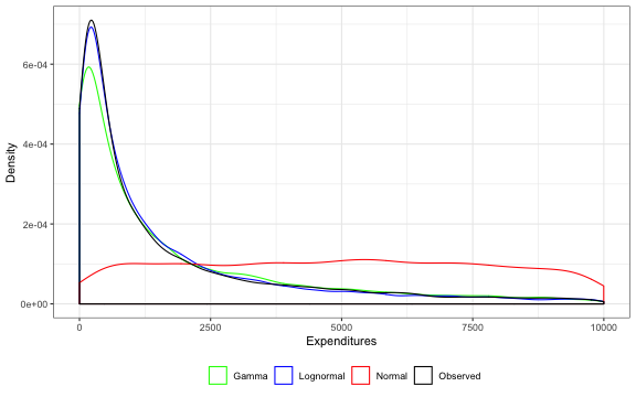
 As expected, the logistic-normal model performs horribly since non-negative expenditures are highly right skewed. The logistic-normal model also allows for negative expenditures which is clearly undesirable since expenditures cannot be negative. The logistic-gamma and logistic-lognormal models both fit the data pretty well although the lognormal model seems to predict the distribution of expenditures slightly better.
We can also compare the quantiles of the simulated distributions to the quantile of the observed data.
MySum <- function(x){
  q <- c(0.30, 0.5, 0.75, .9, .95, .98)
  dat <- c(100 * mean(x == 0, na.rm = TRUE),
           min(x, na.rm = TRUE), quantile(x, probs = q, na.rm = TRUE),
           max(x, na.rm = TRUE))
  names(dat) <- c("PercentZero", "Min", paste0("Q", 100 * q), "Max")
  return(round(dat, 0))
}
sumstats <- rbind(MySum(y), MySum(y.norm),
                  MySum(y.lognorm), MySum(y.gamma))
rownames(sumstats) <- c("Observed", "Normal", "Lognormal", "Gamma")
print(sumstats)
##           PercentZero    Min  Q30 Q50  Q75   Q90   Q95   Q98    Max
## Observed           23      0   92 431 2122  7143 13858 28336 537120
## Normal             23 -47562 -279   0 9736 18873 24143 29893  67423
## Lognormal          23      0   88 462 2052  6896 13642 31036 907396
## Gamma              23      0   35 479 2367  7094 12782 23148 211974
Here we see that the logistic-lognormal model is more accurate at the 30th percentile while simulated data from both the logistic-gamma model and logistic-lognormal model are similar at the upper quantiles. The logistic regression also accurately predicts the proportion of individuals with zero expenditures.
Summary
There is unfortunately no one-size fits all model for healhcare expenditure data. A logistic regression predicts whether expenditures are nonzero well, but models for positive expenditures must be chosen on a case by case basis. If predicting mean costs is the primary goal than an OLS regression on expenditures in levels is straightforward and works pretty well. If an analyst is concerned about making inferences on the regression coefficients, then an OLS regression on the log of expenditures is likely preferable because regression coefficients are more likely to be linear on the log scale than on the raw scale. Lastly, if an analyst wants to predict the entire distribution of expenditures, then both the lognormal and gamma models should be considered.