Bayesian Markov Cohort Models
- Overview
- Parameter Uncertainty in the Markov Model
- Estimating Parameters in JAGS
- Implementing the Bayesian Markov Model
- Decision Analysis
Overview
One problem with a deterministic Markov cohort model is that it does not account for parameter uncertainty. A Bayesian approach provides a natural modeling framework for doing this.
Here, we repeat the HIV example in a Bayesian manner.
Parameter Uncertainty in the Markov Model
There are three sources of parameter uncertainty that the model might account for:
- uncertainty in the transition matrices,
- uncertainty in the relative risk estimates,
- uncertainty in estimated costs.
Chancellor et al. provide information that can be used for the first two parameter types but not the cost estimates.
Transition Matrices
To account for uncertainty about the transition matrices we can use data on counts of transitions from one state to the next. These counts are reported in the “transition table” in the R code below.
tt <- matrix(c(1251, 350, 116, 17,
             0, 731, 512, 15,
             0, 0, 1312, 437),
             ncol = 4, nrow = 3, byrow = TRUE)
The probability of a transition from a given state to any of the other 4 states can then be modeled with a multinomial distribution.
Relative Risk Estimates
Since the relative risk is a ratio it does not follow a normal distribution even if the sample size is large. However, since the log of the relative risk is just a difference in proportions, it is approximately normal if the sample size is reasonably large.
In our case, the estimated relative risk of disease progression is 0.509 (95% CI 0.365 to 0.710). Taking logs, we can calculate the standard error on the log scale.
rr.est <- .509
lrr.est <- log(.509)
lrr.upper <- log(.710)
lrr.se <- (lrr.upper - lrr.est)/qnorm(.975)
Since the log of the relative risk is approximately normal, this suggests that the relative risk follows a lognormal distribution with a mean and standard deviation (on the log scale) of -0.675 and0.17, respectively.
Estimating Parameters in JAGS
We can specify a lognormal distribution for the relative risk and a multinomial distribution for the transition matrices in JAGS. We use a Dirichlet prior distribution, which is a multivariate generalization of the beta distribution and a conjugate prior for a multinomial likelihood function.
model {
# lognormal model for relative risk
  rr ~ dlnorm(mu.lrr, tau.lrr)

# multinomial-dirichlet model for transition matrix
  # priors
    p[1, 1:S] ~ ddirch(alpha[1:S])
    p[2, 1] <- 0
    p[2, 2:S] ~ ddirch(alpha[2:S])
    p[3, 1] <- 0
    p[3, 2] <- 0
    p[3, 3:S] ~ ddirch(alpha[3:S])

  # likelihood
    tt[1, 1:S] ~ dmulti(p[1, 1:S], n[1])
    tt[2, 2:S] ~ dmulti(p[2, 2:S], n[2])
    tt[3, 3:S] ~ dmulti(p[3, 3:S], n[3])
}
Some of the transition probabilities are assumed to be be 0 and there is no need to specify transition probabilities from death to other states (i.e. the 4th row of the transition matrix).
Before estimating the model we must first create the data and specify prior parameters in R. Since there are 4 states, the Dirichlet distribution is parameterized by a vector \(\alpha= (\alpha_1, \alpha_2, \alpha_3, \alpha_4)\); we use an uninformative prior by setting \(\alpha_s\) equal to 1 in each state \(s\). Also, note that the lognormal distribution in JAGS is defined in terms of the precision, that is, as the inverse of the variance.
S <- 4
n <- apply(tt, 1, sum)
alpha <- rep(1, S)
mu.lrr <- lrr.est
tau.lrr <- 1/lrr.se^2
params <- c("rr", "p")
jags.data <- list("mu.lrr", "tau.lrr", "S", "n", "alpha", "tt")
We run 3 chains of 10,000 iterations. The first 5,000 iterations in each chain are discarded and the sequence is thinned by only keeping every 5th draw after burnin, yielding 3,000 random draws from the posterior distribution.
library("R2jags")
set.seed(100)
jagsfit <- jags(data = jags.data, parameters.to.save = params,
                 model.file = "_rmd-posts/markov_cohort.txt", n.chains = 3,
                 n.iter = 10000, n.thin = 5, progress.bar = "none")
We can view output from the model.
print(jagsfit)
## Inference for Bugs model at "_rmd-posts/markov_cohort.txt", fit using jags,
##  3 chains, each with 10000 iterations (first 5000 discarded), n.thin = 5
##  n.sims = 3000 iterations saved
##          mu.vect sd.vect   2.5%    25%    50%    75%  97.5%  Rhat n.eff
## p[1,1]     0.720   0.011  0.699  0.713  0.720  0.728  0.741 1.001  3000
## p[2,1]     0.000   0.000  0.000  0.000  0.000  0.000  0.000 1.000     1
## p[3,1]     0.000   0.000  0.000  0.000  0.000  0.000  0.000 1.000     1
## p[1,2]     0.202   0.010  0.183  0.195  0.202  0.208  0.221 1.001  3000
## p[2,2]     0.580   0.014  0.553  0.571  0.580  0.590  0.607 1.002  1100
## p[3,2]     0.000   0.000  0.000  0.000  0.000  0.000  0.000 1.000     1
## p[1,3]     0.067   0.006  0.056  0.063  0.067  0.071  0.080 1.001  3000
## p[2,3]     0.407   0.014  0.380  0.398  0.407  0.416  0.434 1.002  1400
## p[3,3]     0.750   0.010  0.730  0.743  0.750  0.757  0.770 1.001  2600
## p[1,4]     0.010   0.002  0.006  0.009  0.010  0.012  0.016 1.001  2200
## p[2,4]     0.013   0.003  0.007  0.010  0.012  0.015  0.020 1.001  2200
## p[3,4]     0.250   0.010  0.230  0.243  0.250  0.257  0.270 1.001  2600
## rr         0.516   0.091  0.361  0.451  0.508  0.571  0.722 1.001  3000
## deviance  44.350   3.408 39.665 41.864 43.720 46.136 52.903 1.001  3000
##
## For each parameter, n.eff is a crude measure of effective sample size,
## and Rhat is the potential scale reduction factor (at convergence, Rhat=1).
##
## DIC info (using the rule, pD = var(deviance)/2)
## pD = 5.8 and DIC = 50.2
## DIC is an estimate of expected predictive error (lower deviance is better).
We must combine the posterior draws from the separate chains.
jagsfit.mcmc <- do.call("rbind", as.mcmc(jagsfit))
It is worth noting that although I have used JAGS (mainly because it makes it easy to extend the model), JAGS is not actually needed in this case. Since we used a Dirichlet prior for the multinomial distribution, one can show that the posterior distribution for the Dirichlet-multinomial model follows a Dirichlet distribution with parameters \(\alpha' = (\alpha'_1, \alpha'_2, \alpha'_3, \alpha'_4)\) where \(\alpha'_s = \alpha_s + y_s\) and \(y_s\) is the total number of individuals transitioning to state \(s\).
We can see this in R by considering individuals transitioning from state 1 to state 2. We compare random draws from a Dirichlet distribution with the appropriate posterior parameters and posterior draws from the JAGs model.
library(MCMCpack)
summary(rdirichlet(nrow(jagsfit.mcmc), tt[1, ] + alpha[1])[, 2])
##    Min. 1st Qu.  Median    Mean 3rd Qu.    Max.
##  0.1674  0.1959  0.2019  0.2023  0.2086  0.2362
summary(as.numeric(jagsfit.mcmc[, "p[1,2]"]))
##    Min. 1st Qu.  Median    Mean 3rd Qu.    Max.
##  0.1627  0.1955  0.2017  0.2019  0.2084  0.2410
As expected, the two distributions are essentially identical.
Implementing the Bayesian Markov Model
To implement the Bayesian Markov cohort model we first specify the costs of treatment and quality of life weights in each state.
c.zidovudine <- 2278
c.lamivudine <- 2086.50
c.0 <- c(2756 + c.zidovudine, 3052 + c.zidovudine, 9007 + c.zidovudine, 0)
c.1 <- c(c.0[1:3] + c.lamivudine, 0)
qolw <- c(1, 1, 1, 0)
Then, we write a function that creates transition matrices for each treatment option given transition probabilities and a relative risk.
TMatrix <- function(probs, rr){
  P0 <- matrix(c(probs, rep(0, 3), 1), nrow = 4, ncol = 4, byrow = TRUE)
  P1 <- P0
  P1[upper.tri(P1)] <- P1[upper.tri(P1)] * rr
  P1[1, 1] <- 1 - sum(P1[1, 2:4])
  P1[2, 2] <- 1 - sum(P1[2, 3:4])
  P1[3, 3] <- 1 - sum(P1[3, 4])
  return(list(P0 = P0, P1 = P1))
}
We load in the function MavkovCohort described previously. We use the function to simulate the Markov Model 3000 times using each random draw of the parameters from their posterior distribution.
source("_rmd-posts/markov.R")
ncycles <- 20
delta.c <- rep(NA, nrow(jagsfit.mcmc))
delta.e <- rep(NA, nrow(jagsfit.mcmc))
for (i in 1:nrow(jagsfit.mcmc)){
  tp <- TMatrix(probs = jagsfit.mcmc[i, 2:13], rr = jagsfit.mcmc[, "rr"][i])
  sim0 <- MarkovCohort(P = tp$P0,  z0 = c(1000, 0, 0, 0), ncycles = ncycles,
                       costs = c.0, qolw = qolw,
                       discount = 0.06)
  sim1 <- MarkovCohort(P = c(replicate(2, tp$P1, simplify = FALSE),
                             replicate(ncycles - 2, tp$P0, simplify = FALSE)),
                       z0 = c(1000, 0, 0, 0), ncycles = ncycles,
                       costs = c(replicate(2, c.1, simplify = FALSE),
                                 replicate(ncycles - 2, c.0, simplify = FALSE)),
                       qolw = qolw, discount = 0.06)
  delta.c[i] <- (sum(sim1$c) - sum(sim0$c))
  delta.e[i] <- (sum(sim1$e) - sum(sim0$e))
}
Differences in total costs, \(\Delta_c = c_1 - c_0\) and differences total effects (i.e. life-years), \(\Delta_e = e_1 - e_0\) between combination therapy and monotherapy are saved for each simulated Markov model, which generates a complete probability distribution for each quantity.
Decision Analysis
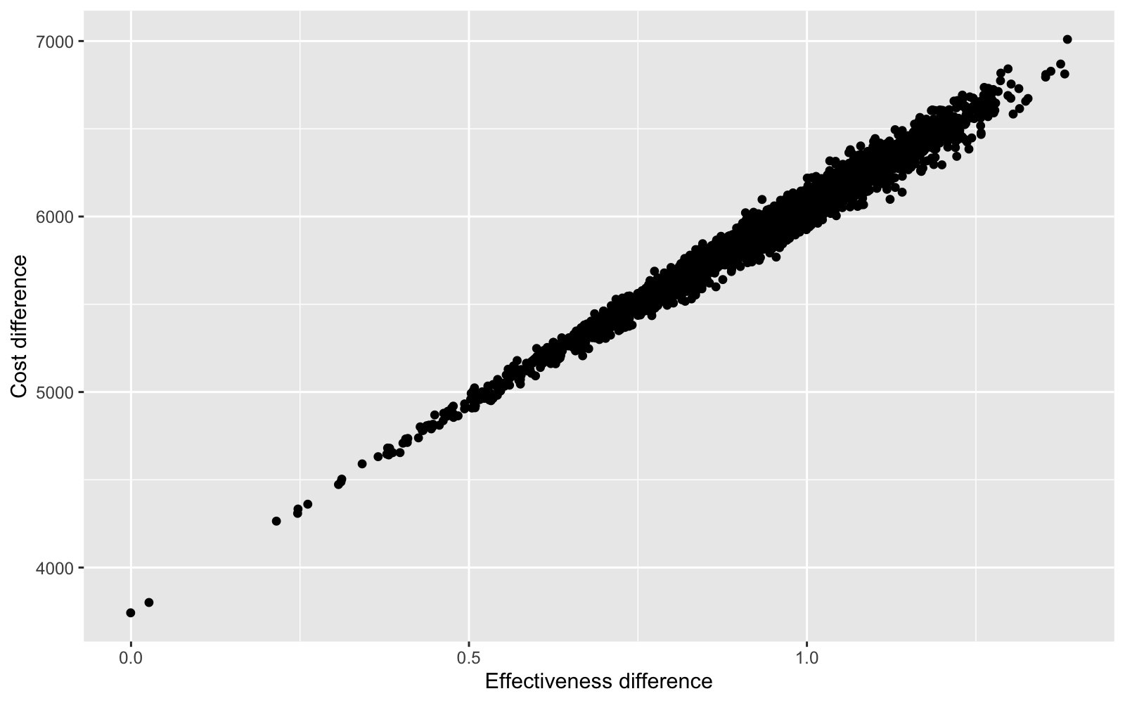
One advantage of a Bayesian approach is that uncertainty can be incorporated into decision analysis. For instance, we can look at the entire distribution of differences in costs and effects using a cost-effectiveness plane.
library("ggplot2")
ce.dat <- data.frame(delta.c = delta.c, delta.e = delta.e)
ggplot(data = ce.dat, aes(x = delta.e, y = delta.c)) + geom_point() +
  xlab("Effectiveness difference") + ylab("Cost difference")

Differences in costs and differences in effects are highly correlated because 1) patients live longer lives (which increases costs) when treatment effects are larger (i.e. the relative risk of disease progression declines), and 2) the model does not account for uncertainty in costs.
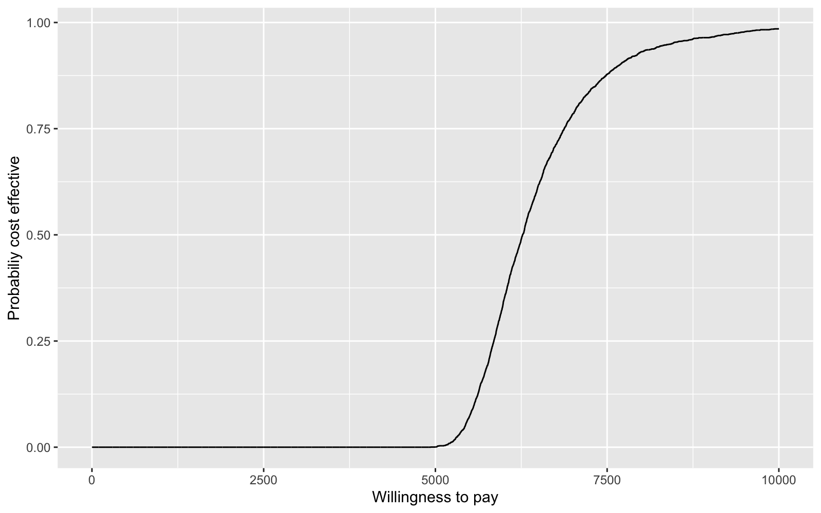
We summarize the uncertainty associated with a decision with a cost-effectiveness acceptability curve (CEAC). If we define \(k\) as the amount that a decision maker is willing to pay for an additional life-year, then the CEAC is,
\[\begin{aligned} Pr\left(k > \frac{\Delta_c}{\Delta_e}\right). \end{aligned}\]For each value of \(k\), we calculate this probability as the fraction of times \(k\) is larger than \(\Delta_c/\Delta_e\) in our posterior distribution. We can plot the CEAC for a range of values of \(k\) to see how cost-effectiveness varies with willingness to pay.
pce <- rep(NA, 10000)
for (k in 1:10000){
  pce[k] <- mean((k * delta.e - delta.c) > 0)
}
ceac.dat <- data.frame(k = seq(1, length(pce)), pce = pce )
ggplot(data = ceac.dat, aes(x = k, y = pce)) + geom_line() +
  xlab("Willingness to pay") + ylab("Probabiliy cost effective")
